Annotated Pen Plots

I’ve posted pictures of my plotter-annotated pieces before, and have gotten some questions about what is being written to the back of each piece. I’ll use this post to describe what’s being annotated in a little more detail. Hopefully you can incorporate some of these tips into your own work!

Organizing physical media

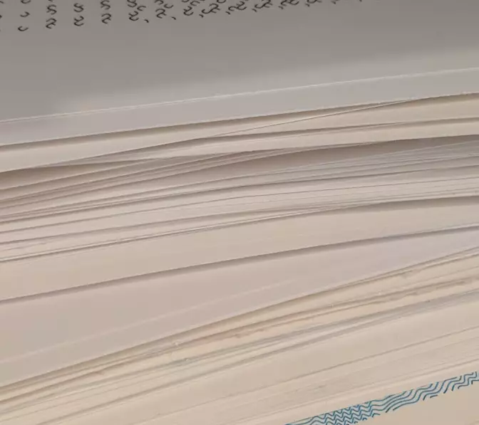
After several months of pen plotting I’ve managed to accumulate quite a thick stack of plots:

To keep track of them I started by checking the plotter file (e.g. an SVG) into version control (git), and writing the date that the plot was created on the back of each piece. This allowed me to go back and easily re-plot any previous work in case a friend or follower wanted a copy for themselves. However, there were a few problems:

• Any parameters used to generate the plot were lost (e.g. particle_count=100, or width=20cm) – the piece could only be re-plotted as-is from the file I saved.
• Tying the date on the back of the plot back to a file in version control became cumbersome as the number of plots grew.
• The date alone wasn’t always enough to tie a sepecific plot to a specific git commit.

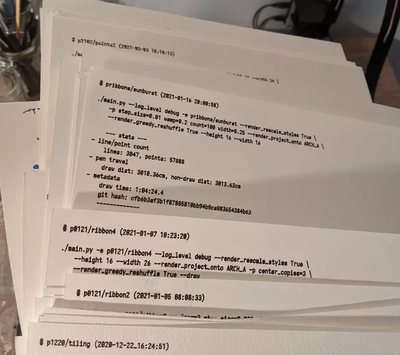
I was able to solve these problems by having the pen plotter write all necessary metadata (and then some) on the back of each plot:

Annotation details

Note: All of these annotations are auto-generated – each time my library drives the plotter, or generates a new piece it records the details shown below. Annotating a plot just requires flipping the paper over, and running a single command. I highly recommend automating this in your own setup if you want to incorporate it into your own workflow!

Let’s break down (a slightly simplified version of) the above annotation:

At the top, I write the identifier for this algorithm (file & function) and when this plot was generated:

 1 | # pribbons/sunburst (2021-01-16 20:00:58)
   :   ^~~~~~~  ^~~~~~~~  ^~~~~~~~~~~~~~~~~~~
   :    file     function  date & time plot was generated

Next, I write the list of command line arguments used to invoke the plotter library including parameters used to drive the algorithm that produced this plotter piece:

 2 | ./main.py -e pribbons/sunburst -p step_size=0.01 wamp=0.2 count=100 \
   :   ^~~~~~~ ^~~~~~~~~~~~~~~~~~~~ ^~~~~~~~~~~~~~~~~~~~~~~~~~~~~~~~~~~~
   :    prog    file/function        plot specific parameters (python kwargs)
   .
 3 |   --render_project_onto ARCH_A --height 16 --width 16
   :   ^~~~~~~~~~~~~~~~~~~~~~~~~~~~ ^~~~~~~~~~~~~~~~~~~~~~
   :    the paper size to plot onto  height & width of contents (in cm)

Finally, I include some stats (mostly for fun) about the piece:

 4 | --- stats ---
 5 | - line/point count
 6 |   lines: 3847, points: 57988
   :   ^~~~~~~~~~~  ^~~~~~~~~~~~~
   :    total lines  total points those lines are broken into
   .
 7 | - pen travel
 8 |   draw dist: 3010.36cm, non-draw dist: 3031.63cm
   :   ^~~~~~~~~~~~~~~~~~~~  ^~~~~~~~~~~~~~~~~~~~~~~~
   :    dist. drawn by pen    dist. traveled while not drawing
   .
 9 | - metadata
10 |   draw time: 1:04:24.4
   :   ^~~~~~~~~~~~~~~~~~~~
   :    total draw time  
   .
11 |   git hash: cfb6b3....
   :   ^~~~~~~~~~~~~~~~~~~~
   :    hash for identifying code revision
   .
12 | -------------

Writing these annotations on the back of each piece has been really useful (and I encourage you to try something similar!):

• I can not only recreate a piece, but also regenerate it with new parameters by reading what I set initially off the back of the plot.
• If I’m curious about some property of a piece (e.g. how many polygons went into some packing of shapes), it’s written on the back.
• It’s oddly satisfying to see all of these annotated pieces in one place!

Addendum: generating the annotations

Note: This is fairly Axidraw specific, but applies to any plotter that can plot SVG files. In fact, using the path representation mentioned below in conjunction with Python svgpathtools should allow this to work with any plotter that can take Cartesian commands.

I generate these annotations by simply generating an SVG of the form:

<svg width="20.0cm" height="20.0cm" xmlns="http://www.w3.org/2000/svg">  
  <text x="0.5" y="0.5" font-family="Monospace" font-size="0.35">
    # pribbons/sunburst (2021-01-16 20:00:58)
  </text>
  ...
</svg>

Next, I convert it to a path representation with Inkscape:

inkscape --actions="EditSelectAll;ObjectToPath;FileSave;FileClose" $FILENAME -g

And run the plotter on the result.