Generating Spectral Paint Curves With ML
2023-04-03Kubelka-Munk (KM) Theory models the color of a mixture of paints by using their spectral properties. As a computer artist, this is really interesting to me because it allows one to mix colors in a way that appears “natural”. For example, mixing blue and yellow paint produces green, but mixing blue and yellow RGB colors produces grey.
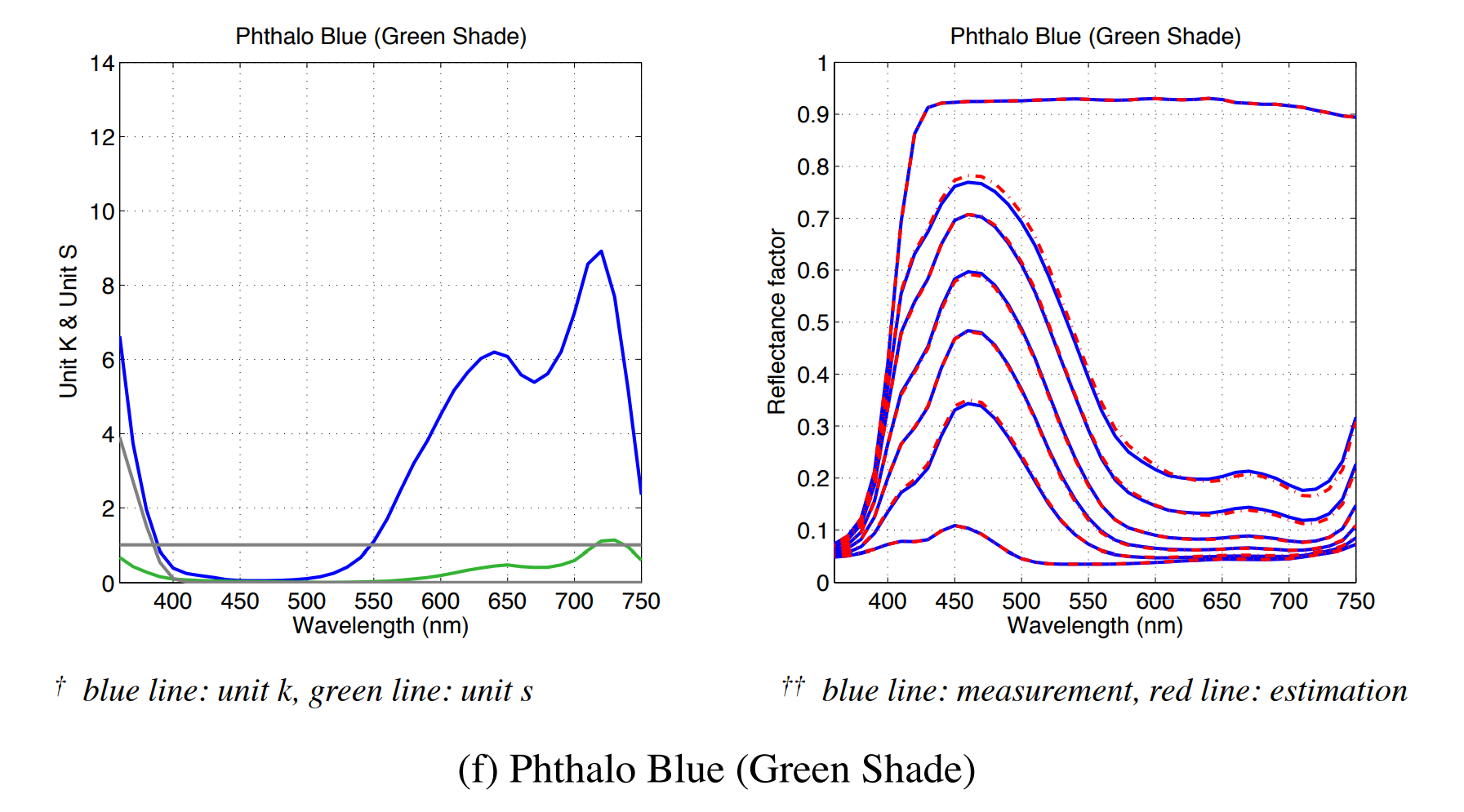
However, applying KM requires knowing the absorption (K) and scattering (S) curves along the visible frequency spectrum for each paint involved. Measuring these values using physical paints is obviously ideal, as the resulting curves should produce very accurate results. This has been done by the lab of Roy Berns in Yoshio Okumura’s thesis: Developing a Spectral and Colorimetric Database of Artist Paint Materials. Unfortunately, the precise values of these curves belong to the paint manufacturer, and are treated as closely-guarded IP. The curves are shown in that thesis, but they lack accurate-enough data to apply KM reliably:
Instead we can try to make “imaginary” curves that don’t fit the shape of real paints, but still mix in interesting ways. It’s possible to do this by hand (and it looks like @ClausWilke is doing this), but it requires shaping curves carefully to produce the desired mixing effects. For example, I naively picked curves that produce blue and yellow on their own, but still mix to produce grey:

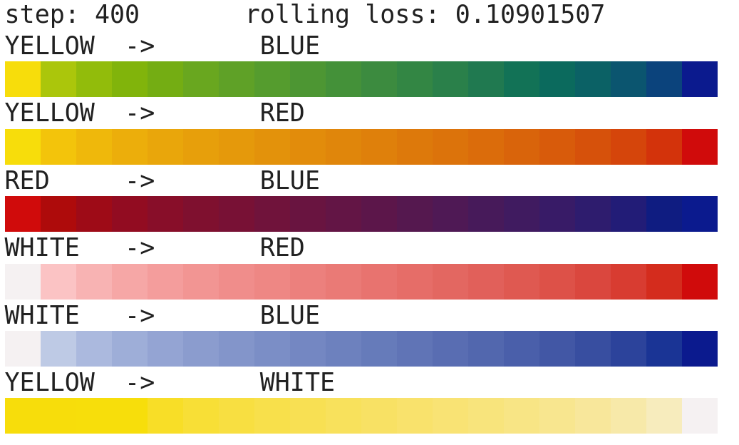
Here I’ll show how to create curves using gradient descent, a machine learning technique, to learn the desired K and S curves for any pigment you can imagine. For example, here is the gradient produced for the learned blue and yellow pigments:

Enter: JAX
JAX is an incredible library for writing automatically differentiable, vectorized GPU code in plain Python and NumPy. It’s intended for machine learning research, but it is much more flexible than TensorFlow or PyTorch, allowing the programmer to write (almost) arbitrary native functions, and differentiate them on the GPU with minimal difficulty.
For the problem of the spectral paint curves we can write the forward-pass (computing a paint mixture using KM, and comparing it to a desired RGB color) in plain Python, and let JAX find the required curves using gradient descent. This is pretty amazing to me.
I’ve implemented a Colab Notebook that does this, which means you can create your own imaginary spectral paint curves from handpicked RGB gradients.
Generating Your Own
To create your own curves you’ll have to run and edit my Notebook.
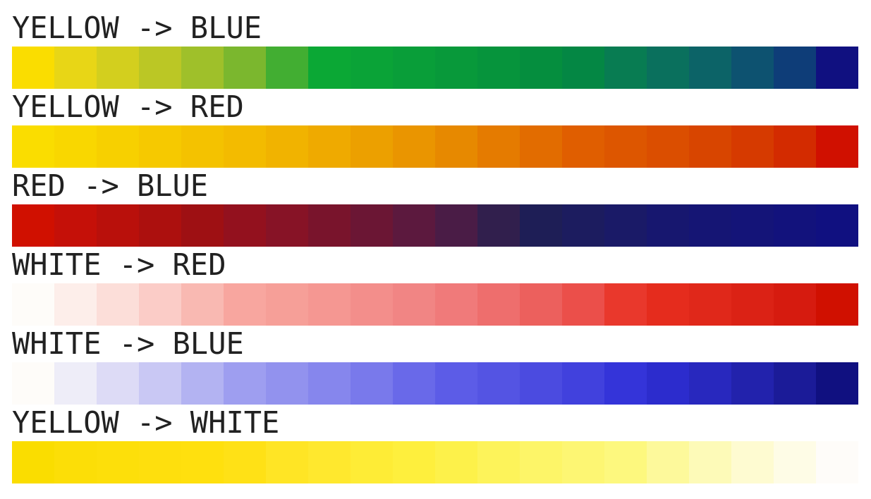
You will need to edit the “Ground Truth Data” section which already contains sample colors and mixing gradients that look like this:
# ...

YELLOW = 0xfadd00
BLUE = 0x101080
RED = 0xd01000
WHITE = 0xfefcf9

save_color('YELLOW', YELLOW)
save_color('BLUE', BLUE)
save_color('RED', RED)
save_color('WHITE', WHITE)

# The final gradients are linearly interpolated using the provided stops.
save_gradient('YELLOW', 'BLUE', [YELLOW, 0x0cab34, 0x038a3f, BLUE])
save_gradient('YELLOW', 'RED', [YELLOW, 0xf0b000, 0xe06000, RED])
save_gradient('BLUE', 'RED', [BLUE, 0x171770, 0x202050, 0x701530, 0xa01010, RED])
save_gradient('WHITE', 'RED', [WHITE, 0xf8a8a0, 0xf08080, 0xe83020, RED])
save_gradient('WHITE', 'BLUE', [WHITE, 0xa0a0f0, 0x6060e8, 0x3030d8, BLUE])
save_gradient('WHITE', 'YELLOW', [WHITE, 0xfcf880, 0xfdf040, 0xffe010, YELLOW])

# ...
Note: it’s important that the first and last stop of each gradient matches the base color it corresponds to for training to converge.
You can train more or fewer paints at once, but if you wish to train more, you’ll need to provide more pair-wise sample gradients. While you don’t need to provide a mixing gradient for every pair of colors, it seems to help training. Not all possible gradients can be represented using KM theory, so be aware that your training may never converge.
The notebook will draw the color gradients you’ve provided like so:
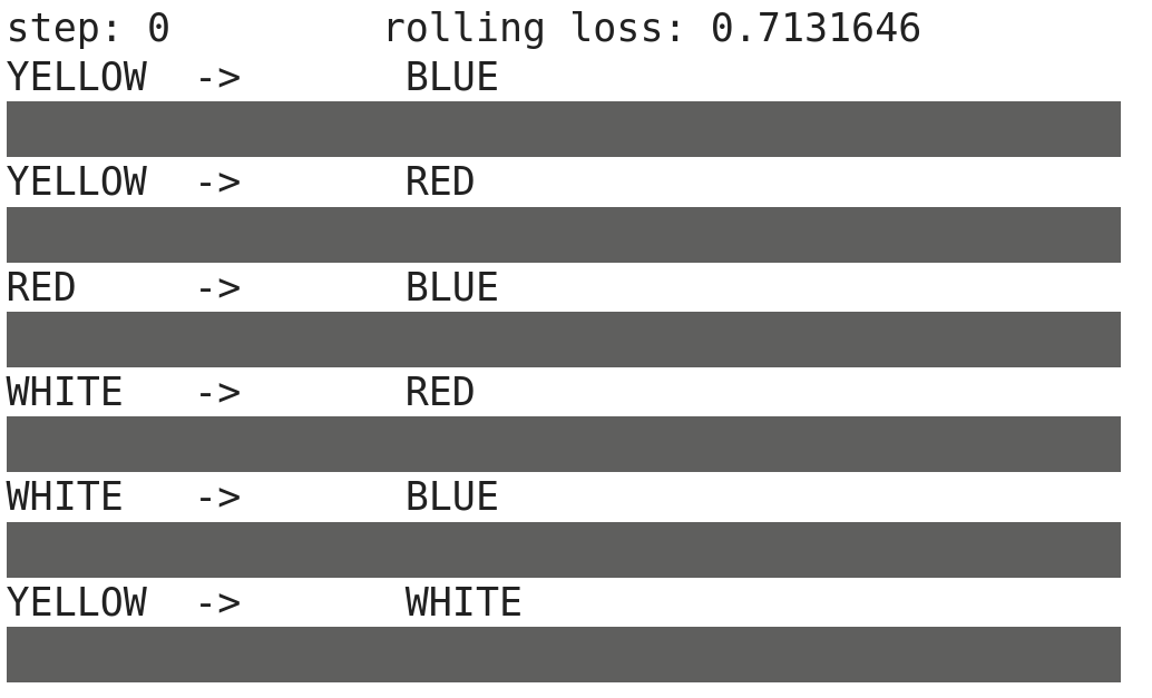
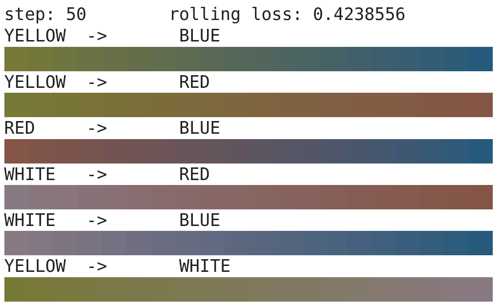
With the desired base paints and their color gradients defined, the training can begin. Note, instead of learning the weights in a neural network (like we typically see in examples of gradient descent), we are learning K and S curves that best satisfy the desired color gradients. There is no neural network being trained here.
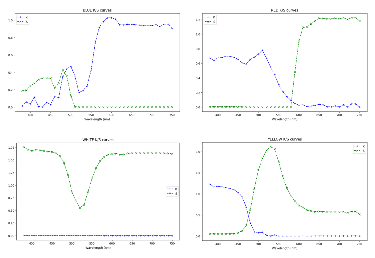
Once training is complete, you can export the generated curves. There is a big difference when comparing the BLUE paint’s curve to the Phthalo Blue Green curve shown at the top of this post. However, the goal wasn’t to learn the “true” representation, but only one that produces pleasing results when mixed with other colors.
Using the Curves
Using the curves is a little bit involved and requires some color science. Fortunately, the Mixbox paper does a fantastic job explaining the process in the “Background and Related Work” section using formulas 1-7.
If you don’t want to implement this by hand, I have an implementation of KM mixing in Python in this Notebook, as well as in GLSL/JavaScript in my Open KM repository.
Enjoy! Please share with me if you use these colors in your work.